Lectures
There is a menu item for each lecture where you can find a reading
guide for the textbook, and links to additional material.
For the lecture locations please look at
timeedit. The
timeedit schedule is always correct. If there are any discrepancies
between this page and timeedit, then please inform me.
Subsections of Lectures
Lecture 1
Today’s Topics: Introduction and asymptotic analysis
- Introduction/revision on algorithm analysis
- Worst case running time.
- Introduction to asymptotic analysis $O$,$\Theta$ and $\Omega$.
Links to Slides and other material
- Slides
on introduction and logistics.
- Slides
on an asymptotic analysis.
Reading Guide
What should I know by the end of this lecture?
- How is the course structured? How do the assignments, help sessions
and labs work?
- What does it mean to analyse an algorithm?
- What is worst case performance?
- What is the definition of $O(f(n))$, $\theta(f(n)$, and
$\Omega(f(n))$?
- What are some of the basic properties of $O()$,$\theta()$, and
$\Omega()$.
Lecture 2
Today’s topics: Divide and Conquer and Algorithm Analysis
- Divide and Conquer, in particular how to derive a recurrence
relation for the running time.
- More on $O$,$\Theta$, and $\Omega$
- The Master theorem and how to apply it.
Slides used
Reading Guide
Chapter 3 and 4 (except 4.6) of
CLRS3
or Chapter 3 and 4 (except 4.6
and 4.7) of
CLRS4.
You might find the following slides useful: Divide and Conquer
I
which has some more examples on algorithm analysis, and
Divide and Conquer
II
that has information on the master theorem.
What should I know by the end of this lecture?
You should know much more about the Big O notation. In particular
- General algebra with $O$, $\theta$ and $\Omega$. For example when
is $O(f(n)) \leq O(g(n))$?
- Constant time $O(1)$.
- Linear time $O(n)$, polynomial time, exponential time
- The rate of different asymptotic growths.
Further you should know about divide and conquer an algorithm design
technique and the Analysis of Divide and Conquer using recurrence
relations. You should understand and be able to reproduce a simple
divide and conquer analysis of an algorithm such as binary search or
merge sort. You should understand how to go from recurrence relations
such as
$$
T(n) = aT(n/b) + f(n)
$$
to asymptotic analysis of the function $T(n)$. For which functions $g$
is the following statement true:
$$
T(n) \in O(g(n))
$$
Although I do not expect expect you understand the proof, you should
try to get an intuition of the different cases of the master theorem.
Lecture 3
Guest Lecture by Frej Knutar Lewander
Today’s topic: Graphs revision
Slides
Reading Guide
- Chapter 22, except 22.4 of CLRS3 or
Chapter 20, 20.1-20.3 of
CLRS4.
- Chapter 24 Pages 643-650 and Section 24.3 of
CLRS3
or chapter 22 (22.1, 22.2
22.3) of CLRS4.
What should I know by the end of this lecture?
- What did I forget from my previous courses?
- What is a graph? What is a digraph?
- What is a good API for graphs?
- How can they be represented?
- Depth-first and breadth-first search.
Lecture 4
Today’s topic: Dynamic Programming
- Dynamic programming. Introduction.
Slides
- The slides can be found here
Reading Guide
- Chapter 15, 15.1, 15.2 ,15.3, 15.4 of
CLRS3
or Chapter 14, 14.1 , 14.2, 14.3 and 14.4 of
CLRS4.
What should I know by the end of this lecture?
- What is dynamic programming? Simple example dynamic programming as
Memorisation.
- Some example dynamic programs.
Lecture 5
Today’s topic: Dynamic Programming
- More on Dynamic Programming, Knapsack and an example.
- Pseudo Polynomial vs. Polynomial.
Links to Slides
- The slides can be found here
Reading Guide
All of Chapter 15 of
CLRS3 or all of
Chapter 14 of
CLRS4.
The textbook does not say that much about pseudo-polynomial time and
the 0-1 Knapsack problem, even though it is an important
concept. There there is plenty of material on the internet. I suggest
that you start with the Wikipedia entries on Pseudo-polynomial
time and the
Knapsack
problem. You also
might find these
notes
useful.
What should I know by the end of this lecture?
- Yet more dynamic programming examples
- How to decompose a problem using Dynamic Programming
- Optimal substructure
- The difference between polynomial and pseudo-polynomial time. Ask
yourself why isn’t the dynamic program for 0-1 Knapsack polynomial
time?
Lecture 6
Today’s topics: Greedy Algorithms
- Introduction to Greedy Slides
1-15.
- We will look a greedy algorithm for the coin-change problem. This only
works with certain denomination coins. You should understand the
proof of why it works, and when it works.
- Interval scheduling. Again we met a dynamic programming solution
before, here we will look at a simple greedy algorithm and
understand why it is correct.
- Shortest Paths as a greedy algorithm. Slides 1-16
- All-Pairs Shortest path using Dynamic programming (The
‣ Bellman–Ford–Moore algorithm). Slides
33-41
Reading Guide
- Chapter 16 except 16.4 and 16.5 of
CLRS3
or Chapter 15, 15.1,15.2 and
15.3 of
CLRS4.
What should I know by the end of this lecture?
- How do I set up shortest paths as a dynamic program? How do I avoid cycles?
- How does Dijkstra’s algorithm work? Why is it correct?
- What is a greedy algorithm?
- How do greedy algorithms compare with dynamic programming?
- Are Greedy algorithms always optimal?
Lecture 7
Today’s topics: Minimal Spanning Trees.
Reading Guide
What should I know by the end of this lecture?
- What is a minimal spanning tree?
- Why is the greedy algorithm correct?
- How does Prim’s Algorithm work?
Lectures 8,9
Network Flows
When I do these lectures live, it normally takes me 3 lectures to go
through the material slowly and do lots of examples. This is a list
of topics that are needed to under network flows. You goal should be
to understand each topic.
- Definition of flow network.
- The minimum-cut problem.
- The maximum flow problem.
- The definition of a residual network.
- An Augmented path.
- The statement of the Min-cut, max-flow theorem.
- The Ford–Fulkerson algorithm.
- How to use the max-flow algorithm for maximum bipartite matching.
Lecture 8
Lecture 9
Alternative mathematical API. Flows that are Skew Symmetric flows,
that is $f(u,v)= -
f(v,u)$. We’ll do this on the blackboard, but skew symmetric flows
are a bit counter intuitive, but they make the proofs and
implementation easier. Take a look at the presentation at
Wikipedia. This
is not examined, and I won’t go into much detail.
Min-Cut Max-Flow duality slides 25-36 of
NetworkFlow
I
Bipartite matching slides 1-17 of NetworkFlow
II.
Reading Guide
- Chapter 26, except 26.4 and 26.5 of
CLRS3
or Chapter 24 of
CLRS4.
What should I know by the end of this set of lectures?
- Do I understand the definitions of a flow network, min-cuts and
maximum flows?
- Why does the naive greedy algorithm for maximum flow fail?
- The relation between augmented paths and residual networks.
- What is the relationship between flows and cuts?
- What is the relationship between negative flows and residual
networks?
- What does the min-cut max-flow algorithm tell us and how does it
help us to derive an algorithm?
- What is bipartite matching? What are its applications?
Lectures 10 and 11
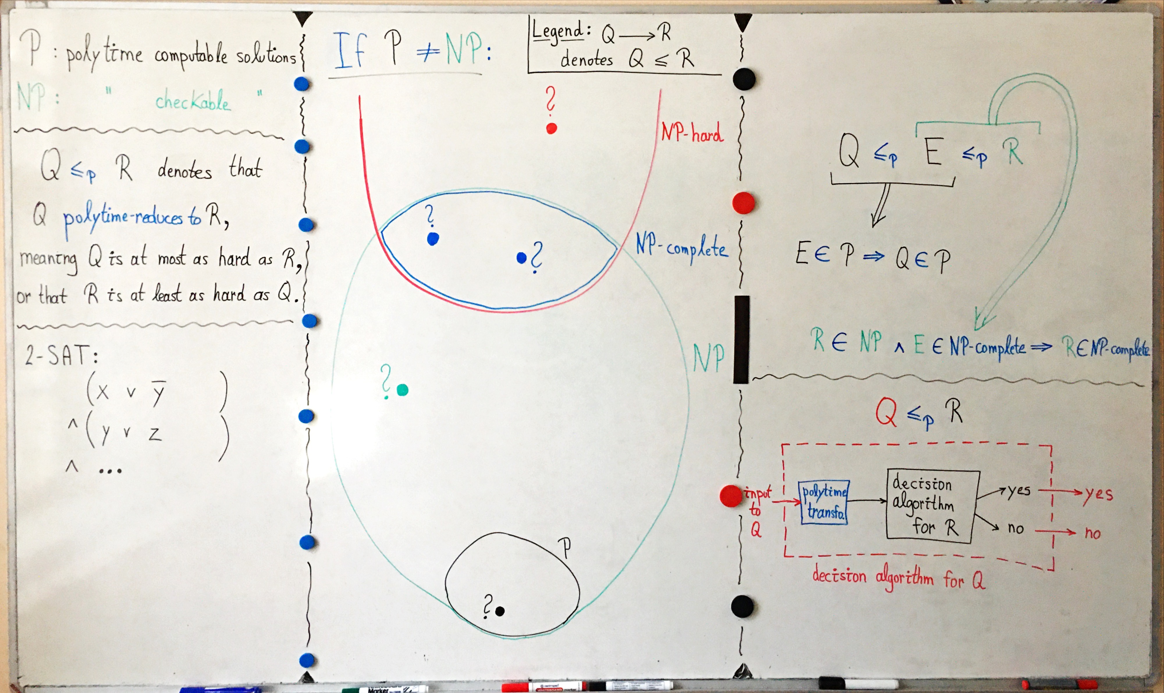
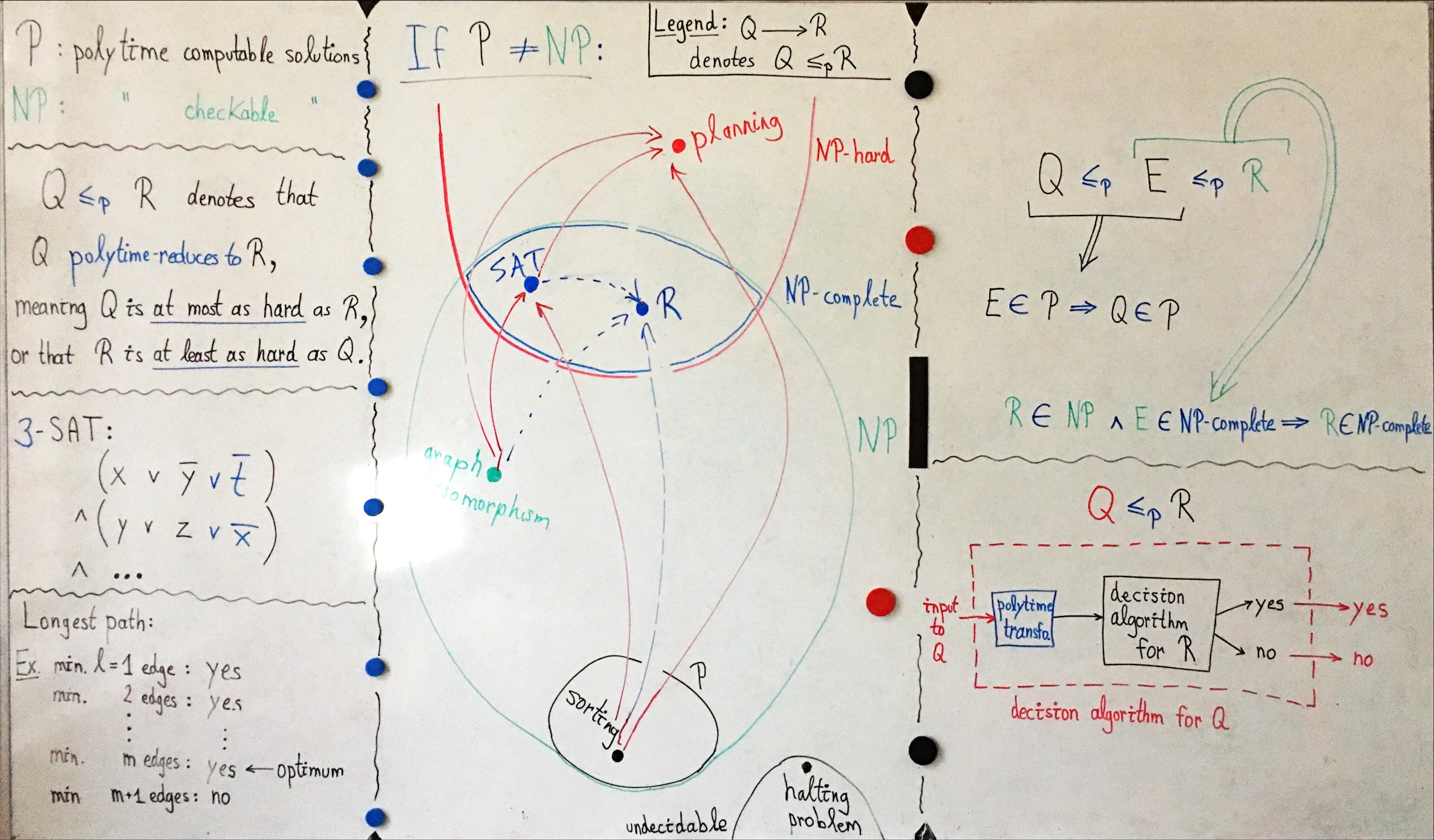
Today’s topic: P vs NP
This will be a not so formal introduction to P and NP. Every computer
scientist should know something about NP complete problems. If you
know that a problem is NP complete, then you know that it is very hard
to find an optimal solution.
- The definition of P and NP
- The definition of Reduction and NP Hardness
- NP Completeness
- Some NP Complete Problems.
- What now? What courses should I take to learn more about algorithms
and optimisation?
This material is examined.
Links to Slides and other material.
These lectures will given by Pierre
Flener.
The slides for the lecture can be found here
Reading Guide
What should I know by the end of this set of lecture?
- The definition of NP? What has guessing a solution got to do with
complexity?
- How do reductions work?
- What is a complete problem for a complexity class?
- You should know some NP-complete problems and have enough idea about
how reductions work so that you can decide if your problem is
NP-complete or not.
Lecture 12
Today’s topic: Union Find
- Disjoint-set data-type. What is the API and some applications?
- Naive representation: Sets represented as trees.
- Representing trees as arrays, and Naive linking.
- Link by Size
- Link by Rank
- Path compression
- Analysis of run time.
Slides
I used slides 1 to 41 from
UnionFind.
Reading Guide
- These notes
contain useful information on greedy algorithms in general and section
5.1.4 is on Union Find. The best source is the textbook Chapter 21
(excluding section 21.4) of
CLRS3
or
Chapter 19 (excluding 19.4) of CLRS4.
Link to online lectures for further study.
Both William
Fist and
Josh Hug
cover the same material, although Josh Hug takes it much more slowly.
What should I know by the end of this set of lecture?
What is the union-find API?
What are some of the applications of union-find?
How can I use trees to represent sets?
How do I represent sets of trees as a forest?
What are the different strategies for combining trees? Link by Size
and Link by Rank.
What is path compression? How does this improve the complexity of
union-find? Note that if you go deeply into the analysis of
union-find you will come to amortised analysis. This is the
analysis of the complexity of an algorithm over
multiple-runs. Amortised analysis is not part of this course, but
it is part of AD3 -
1DL481
that is normally taught by Pierre
Flener
Lecture 13
Today’s topic: String Matching
- The Rabin-Karp algorithm for fast string matching.
Slides
Reading Guide
- Chapter 32 except sections 32.3 and 32.4 of
CLRS3
or CLRS4.
What should I know by the end of this set of lecture?
- How does Rabin-Karp work? What is the clever idea with
hash-functions.
- How does Rabin-Karp compare with brute force string matching?